[딥러닝] 패션 이미지 데이터 분류

import numpy as np
import pandas as pd
import matplotlib.pyplot as plt
from tensorflow.keras.datasets import fashion_mnist

data = fashion_mnist.load_data()

(X_train, y_train),(X_test, y_test) = data

y_train_one_hot = pd.get_dummies(y_train)
y_test_one_hot = pd.get_dummies(y_test)

from sklearn.model_selection import train_test_split

X_train, X_val, y_train_one_hot, y_val_one_hot = train_test_split(X_train,
                                                                  y_train_one_hot,
                                                                  random_state=3
                                                                  )
                                                                  
from tensorflow.keras import Sequential
from tensorflow.keras.layers import Dense, Flatten
# Flatten : 데이터를 1차원으로 자동적으로 펴주는 역할을 하는 모듈

model = Sequential()

model.add(Flatten(input_shape=(28,28)))

# 입력층 + 중간층 (X_train의 특성 개수를 입력)
model.add(Dense(500, input_dim=784, activation='relu'))

# 중간층
model.add(Dense(300, activation='relu'))
model.add(Dense(100, activation='relu'))

# 출력층 뉴런의 개수는 원핫인코딩 된 컬럼 개수
model.add(Dense(10, activation='softmax'))

model.summary()

Model: "sequential_3"
_________________________________________________________________
 Layer (type)                Output Shape              Param #   
=================================================================
 flatten_3 (Flatten)         (None, 784)               0         
                                                                 
 dense_12 (Dense)            (None, 500)               392500    
                                                                 
 dense_13 (Dense)            (None, 300)               150300    
                                                                 
 dense_14 (Dense)            (None, 100)               30100     
                                                                 
 dense_15 (Dense)            (None, 10)                1010      
                                                                 
=================================================================
Total params: 573,910
Trainable params: 573,910
Non-trainable params: 0
_________________________________________________________________

 

 

# 학습 및 평가방법 설정
# categorical_crossentropy : 다중분류에 사용하는 손실함수
model.compile(loss='categorical_crossentropy',
              optimizer='Adam',   # 최적화함수 : 최근에 가장 많이 사용되는 일반적으로 성능이 좋은 최적화함
              metrics=['acc']    # metrics : 평가방법을 설정(분류문제이기 때문에 정확도를 넣어줌)
              )
              
# 학습
h = model.fit(X_train, y_train_one_hot, validation_data=(X_val, y_val_one_hot),
              epochs=50,
              batch_size=128
              )

plt.figure(figsize=(15,5))

plt.plot(h.history['acc'], label='acc')

plt.legend()
plt.show()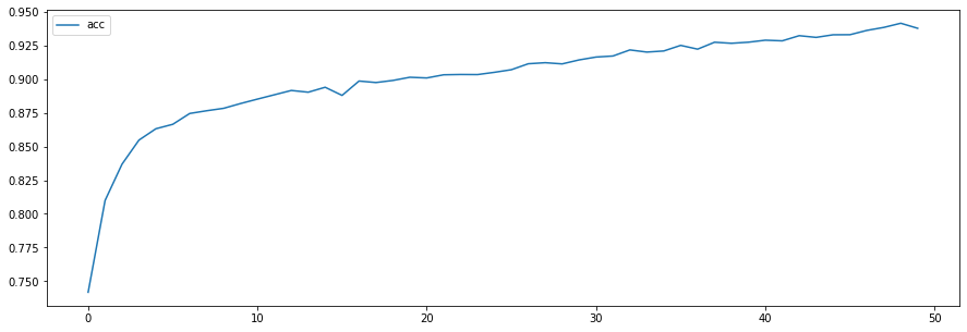

 

plt.figure(figsize=(15,5))

# train 데이터
plt.plot(h.history['acc'],
         label='acc',
         c = 'blue',
         marker='.'
         )

# val 데이터
plt.plot(h.history['val_acc'],
         label='val_acc',
         c = 'red',
         marker='.'
         )

plt.xlabel("epochs")
plt.ylabel("accuracy")

plt.legend()
plt.show()

 

model.evaluate(X_test, y_test_one_hot)

313/313 [==============================] - 1s 3ms/step - loss: 0.5675 - acc: 0.8734
[0.5674822926521301, 0.8733999729156494]